Observing with TolTEC
Overview
Here are the key features of the camera.
| Wavelength | Beamsize (FWHM) | Number of Pixels | Number of Detectors | Maximum Mapping Speed Prediction | Minimum Mapping Speed Prediction |
|---|---|---|---|---|---|
| 2.0mm | 9.5 arcseconds | 586 | 1172 | 69 deg2/mJy2/hr | 10 deg2/mJy2/hr |
| 1.4mm | 6.3 arcseconds | 1266 | 2532 | 20 deg2/mJy2/hr | 3 deg2/mJy2/hr |
| 1.1 mm | 5 arcseconds | 2006 | 4012 | 12 deg2/mJy2/hr | 2 deg2/mJy2/hr |
Since some find these mapping speed units to be awkward, there is simplified integration time calculator that we hope will be useful for those who want to explore TolTEC's ability to map a field to their desired depth.
Alternatively, after reading though this webpage you may be inspired to use the TolTEC Observation Planner which is a more in-depth calculator of field coverage and depth for different observing configurations.
The remainder of this webpage walks through the process of going from an observation concept to calibrated science images with TolTEC. We focus the discussion on producing total intensity maps (Stokes I) and will add more to this description as we fully develop the same processes for making polarized images.
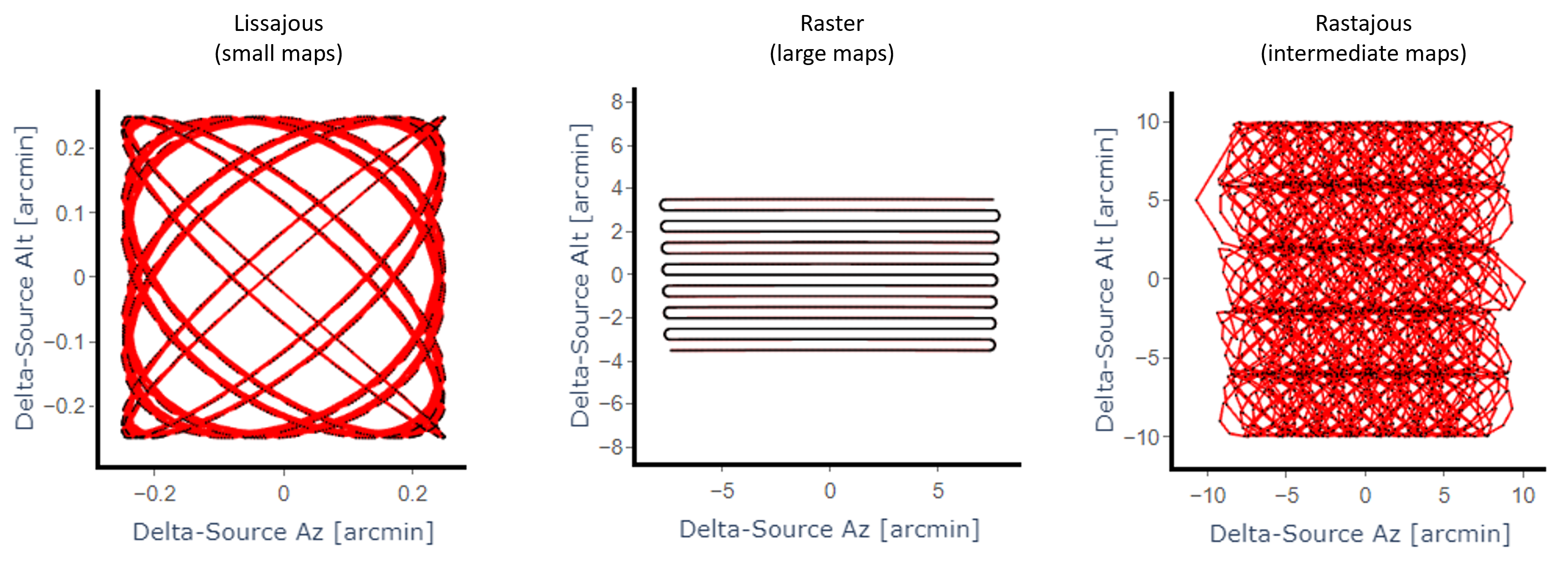
We have implemented a "double-lissajous" pattern to allow Lissajous-style maps to be made on scales larger than 4 to 6 arcminutes diameter. We are still working on finding the best sets of parameters for this observing mode.
Lissajous and Double Lissajous maps can be explored using the TolTEC Observation Planner. Both mapping patterns can be implemented in either the Az/El frame or the Ra/Dec frame.
If we take 5s as a typical turnaround time, the useful observing time during the scan is t_scan = scan length/scan velocity; and the observing efficiency can be estimated by t_scan/(t_scan+5s).
We recommend scan speeds above 50"/s for Raster Maps. We do not know, at this time, what the maximum usable scan speed of the telescope is but we do plan to try to measure this in the fall of 2021. The AzTEC camera was able to usefully map at speeds of 200"/s but was ultimately limited by AzTEC's detector readout rate. The TolTEC readout is 8x that of AzTEC and so we expect a much higher limit to the useful scan speed.
Raster mapping parameters can be explored on the TolTEC Observation Planner.
Rastajous mapping parameters can be explored on the TolTEC Observation Planner. Note that the Rastajous uses the Double Lissajous parameter set and so one might want to set the x_length_1 and y_length_1 to zero to simplify things.
We often use the SMA Calibrator List to choose pointing sources.
Users of TolTEC are only required to choose pointing targets and structure their science field observations so that pointing observations can be made roughly every 45 minutes to an hour apart. The TolTEC pipeline will automatically account for the measured offsets as a part of the standard data reduction process.
TolTEC calibration observations, also known as beammaps, will occur one to two times per night of observing. A beammap is a very finely spaced Raster Map of a target with known mm-flux. A separate map of the target is made with each of the 7715 detectors from which we extract the relative detector locations in the array, the PSFs of the detectors, and a conversion factor from their raw output to flux units (their responsivities). All calibration observations will be carried out by LMT observers and will be shared across multiple TolTEC projects.
A publicly available database of TolTEC pointing, focus, and calibration measurements will be available on an ongoing basis. All data products used for calibration will be accessible through the toltec-calib repository on GitHub which is a part of the toltec-astro git. The toltec-calib data products are designed to be read by the TolTEC-specific softare. We plan to make a more user-friendly web interface in the future.
As of the summer of 2021, the TolTEC team is completing a full instrument simulator that will allow us to explore atmosphere removal techniques and to explore optimal observing approaches for removing the atmosphere and preserving large scale astronomical emission.
Successful proposers will be assigned a Project ID which is unique to their observing program. Projects are sub-divided by distinct Targets that require different sets of Observations to be observed. For TolTEC, an Observation is the atomic unit of a project and each observation is assigned a unique Obsnum. Multiple Observations coadded together result in a set of maps of a Target, and one or more Targets make up a Project.
Successfull proposers will work with LMT staff to develop their observing scripts and plan out their observations. The TolTEC Observation Planner provides an option to output a script that is compatible with the telescope's Monitor and Control system, and so is a good place to start when making your initial plan.
TolTEC currently has one data reduction engine called citlali. Citlali is closely modeled after AzTEC's data reduction engine, macana, but is both much faster and much more flexible. Macana and Citlali are based on the algorithms described in Wilson et al. 2008 and Scott et al. 2008. As a result, we expect Citlali to work well out of the box but also to mature and evolve quickly as the first season of data is reduced. That said, we are working on additional data reduction engines - namely, a maximum likelihood mapmaker - in order to improve our ability to recover extended emission in the maps. This work is ongoing.
All of the TolTEC data reduction software is (or soon will be) publicly available at our TolTEC GitHub. However, due to the complexity of the software and the wide disparity in compute setups, our team will not support troubleshooting the installation of the software for the general public. There are installation guides for each sub-system of the software framework on the GitHub site. From there, if you want to reduce your own data, you are on your own. Instead, we strongly recommend that teams with TolTEC data work closely with LMT or TolTEC team members to have the data reduced on the TolTEC cluster. We are actively building a new web-based interface to our data reduction facilities and we hope to have that live in the fall of 2021.
For targets that require multiple observations, Citlali will perform a weighted coaddition of the observations and, optionally, apply either a Wiener filter constructed from the coadded kernel map and the noise power spectral density, or a simple low-pass filter with a user-defined cut-off. In addition to the above maps, the output data products will include:
Planning an Observation
Pointing, Focus, and Calibration

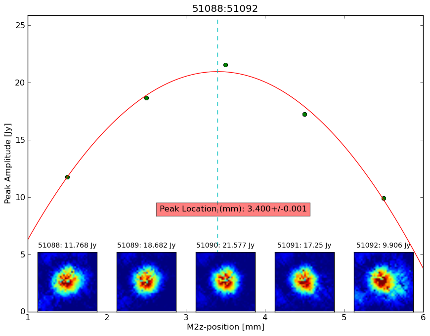 Focusing the LMT is done on an as-needed basis by the telescope observers by monitoring the results of the pointing maps as each night progresses. The image to the left shows a typical focus set made with AzTEC and we plan to use the same approach with TolTEC.
Intrinsic Filtering of Astronomical Signals
Scheduling and Carrying Out Observations
TolTEC Data Reduction
Data Products
Image Name
No. of Images
Units
Description
Signal Maps: I (opt: Q,U)
3 (9)
MJy/sr
Total intensity (and optionally, Stokes Q and U) flux maps from each of the 3 arrays.
Weight Maps: I (opt: Q,U)
3 (9)
(MJy/sr)-2
Weight maps for I (and optionally, Stokes Q and U) for each of the 3 arrays.
Kernel Maps: I (opt: Q,U)
3 (9)
unitless
Filtered represenations of the PSF or user defined kernel shape
Signal to Noise Maps: I (opt: Q,U)
3 (9)
unitless
This is just signal maps * sqrt(weight maps)
Noise Realizations: I (opt: Q,U)
User defined x 3 (9)
MJy/sr
Jackknifed noise realization I (optionally Q and U) maps from each of the 3 arrays.
Image Name (Coadded Observations)
No. of Images
Units
Description
Coadded Signal Maps: I (opt: Q,U)
3 (9)
MJy/sr
Total intensity (and optionally, Stokes Q and U) flux maps from each of the 3 arrays.
Coadded Weight Maps: I (opt: Q,U)
3 (9)
(MJy/sr)-2
Weight maps for I (and optionally, Stokes Q and U) for each of the 3 arrays.
Coadded Kernel Maps: I (opt: Q,U)
3 (9)
unitless
Filtered represenations of the PSF or user defined kernel shape
Coadded Signal to Noise Maps: I (opt: Q,U)
3 (9)
unitless
This is just coadded signal maps * sqrt(coadded weight maps)
Coadded Noise Realizations: I (opt: Q,U)
User defined x 3 (9)
MJy/sr
Jackknifed noise realization I (optionally Q and U) maps from each of the 3 arrays.
and by the Large Millimeter Telescope Project.
This site design is based on a TEMPLATED template.